
You plan your warehouse network according to the demand forecast. But because the forecast is never exact, you keep a safety margin and plan each warehouse to 95% of its capacity. That is not wrong. In a calm market, with forecasts that miss by about 15%, a 95% margin is practically optimal. On our test data, it costs nothing extra in the median and at most 4% in the worst case.
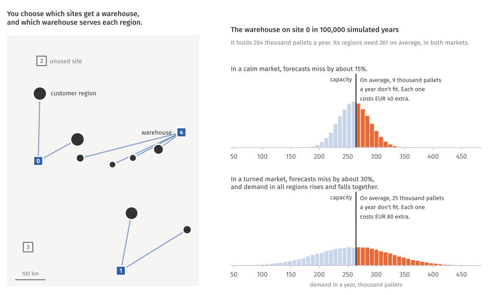
But that margin was learned in a calm market. Suppose the market suddenly changes. Your forecasts now miss by about 30%, and on top of that, the regions you serve are correlated, that is, demand there rises and falls in step. Those pallets that don't fit into your warehouses go to a third-party logistics provider. With demand for its services higher, that provider now charges twice as much as before. The same 95% safety margin then costs a median 14.5% more per year than the plan Quicopt finds, and as much as 36% more in the worst of our 20 test networks. Even with a 90% margin, it is still 6.7% more. Planning with the demand forecast alone does worse still, even when a solver proves the plan optimal. In the median, that plan costs 18% more, and it costs almost 50% more than the solver promised.
Quicopt builds the forecast error directly into the plan. You tell it how far demand may stray from the forecast. Quicopt then chooses the warehouse network that is cheapest across all possible outcomes, and tells you exactly what that network will cost (to within 2% in our tests, which is excellent given the forecast error). When the market changes, you only need to update the forecast parameters instead of re-learning a margin.
Below we plan all 20 test networks both ways, in the calm and in the turned market, with code you can run yourself.
Twenty warehouse networks
Each of the 20 networks has five sites where you could run a warehouse and eight customer regions, spread over a map of 600 × 800 km. Each region is served from exactly one warehouse. A year's cost has three parts:
- a fixed cost for every warehouse you run;
- transport, priced by distance and by each region's demand that year;
- a premium for overflow.
Overflow is the part of a year's demand that a warehouse cannot hold. It goes to a third-party logistics provider, who charges a premium per pallet.
We draw the 20 networks at random, each from a fixed seed, so you can reproduce every number on this page. Demand and capacity are in thousand pallets a year, costs in thousand EUR a year. Network 11 is the one we look at in detail: of the 20 test networks, it is the one where planning for the forecast goes worst once the market turns.
import numpy as np

SITES, REGIONS = 5, 8
TRANSPORT = 0.02          # EUR per pallet and km


def network(number):
    """Network `number`: distances between sites and regions, each region's
    forecast, and each site's capacity and fixed cost."""
    rng = np.random.default_rng(number)
    site_xy = rng.uniform([0, 0], [600, 800], (SITES, 2))        # km
    region_xy = rng.uniform([0, 0], [600, 800], (REGIONS, 2))
    return {
        "distance": np.linalg.norm(site_xy[:, None, :] - region_xy[None, :, :], axis=2),
        "forecast": rng.uniform(60, 140, REGIONS),      # thousand pallets a year
        "capacity": rng.uniform(200, 350, SITES),       # thousand pallets a year
        "fixed_cost": rng.uniform(800, 1200, SITES),    # thousand EUR a year
    }


networks = [network(number) for number in range(20)]

shown = networks[11]
print("site  capacity  fixed cost")
for s in range(SITES):
    print(f"{s:4}  {shown['capacity'][s]:8.0f}  {shown['fixed_cost'][s]:10.0f}")
print("\nregion  forecast")
for r in range(REGIONS):
    print(f"{r:6}  {shown['forecast'][r]:8.0f}")
site  capacity  fixed cost
   0       264         887
   1       222         813
   2       301         880
   3       230         938
   4       335         988

region  forecast
     0        79
     1       124
     2       129
     3        70
     4        97
     5        82
     6        67
     7       132
Two markets
A market, on this page, is three numbers. The forecast error says how far a region's yearly demand typically strays from its forecast (one standard deviation). The correlation says how strongly demand in the regions rises and falls together. The overflow premium is the third-party logistics provider's price per pallet.
In the calm market, your forecasts miss by about 15%, the regions are independent of each other, and overflow costs EUR 40 per pallet. In the turned market, forecasts miss by about 30%, any two regions are correlated at 0.5, and overflow costs EUR 80 per pallet.
We judge every plan by its real cost. That is its average yearly cost over 100,000 simulated years of the market it faces.
calm = {"error": 0.15, "correlation": 0.0, "overflow": 40.0}
turned = {"error": 0.30, "correlation": 0.5, "overflow": 80.0}


def years(net, market, n, seed):
    """`n` simulated years of demand: one row per year, one column per region."""
    rng = np.random.default_rng(seed)
    own = rng.standard_normal((n, REGIONS))     # each region's own swing
    shared = rng.standard_normal((n, 1))        # the swing all regions share
    rho = market["correlation"]
    swing = np.sqrt(1 - rho) * own + np.sqrt(rho) * shared
    return np.maximum(net["forecast"] + market["error"] * net["forecast"] * swing, 0.0)


def yearly_cost(net, market, plan, demand):
    """The cost of `plan` in each simulated year: fixed costs, transport, overflow."""
    open_sites, serves = plan
    transport = (TRANSPORT * net["distance"][serves, np.arange(REGIONS)] * demand).sum(axis=1)
    load = np.zeros((len(demand), SITES))
    for r in range(REGIONS):
        load[:, serves[r]] += demand[:, r]
    overflow = np.maximum(load - net["capacity"] * open_sites, 0.0).sum(axis=1)
    return net["fixed_cost"] @ open_sites + transport + market["overflow"] * overflow


def real_cost(number, market, plan):
    """The plan's average yearly cost over 100,000 simulated years."""
    net = networks[number]
    return yearly_cost(net, market, plan, years(net, market, 100_000, seed=number + 2000)).mean()
Planning for the forecast
The usual way to plan the network is a mixed-integer linear program (MILP). It chooses which warehouses to run and which warehouse serves each region, so that the cost is lowest if every region's demand equals its forecast. HiGHS, an open-source solver, solves it and proves the plan optimal.
import pyomo.environ as pyo


def plan_for_forecast(number, market, margin=1.0):
    """The network that is cheapest if every region's demand equals its forecast,
    proven optimal by HiGHS. With a margin below 1, each warehouse counts as
    holding only that share of its capacity. Returns the plan and the cost the
    solver promises."""
    net = networks[number]
    m = pyo.ConcreteModel()
    m.open = pyo.Var(range(SITES), domain=pyo.Binary)                    # run a warehouse at site s?
    m.serve = pyo.Var(range(SITES), range(REGIONS), domain=pyo.Binary)   # does site s serve region r?
    m.over = pyo.Var(range(SITES), domain=pyo.NonNegativeReals)          # overflow at site s
    m.once = pyo.Constraint(range(REGIONS), rule=lambda m, r: sum(m.serve[s, r] for s in range(SITES)) == 1)
    m.only_open = pyo.Constraint(range(SITES), range(REGIONS), rule=lambda m, s, r: m.serve[s, r] <= m.open[s])
    m.overflow = pyo.Constraint(range(SITES), rule=lambda m, s: m.over[s] >= sum(
        net["forecast"][r] * m.serve[s, r] for r in range(REGIONS)) - margin * net["capacity"][s] * m.open[s])
    m.cost = pyo.Objective(sense=pyo.minimize, expr=(
        sum(net["fixed_cost"][s] * m.open[s] for s in range(SITES))
        + sum(TRANSPORT * net["distance"][s, r] * net["forecast"][r] * m.serve[s, r]
              for s in range(SITES) for r in range(REGIONS))
        + market["overflow"] * sum(m.over[s] for s in range(SITES))))
    solver = pyo.SolverFactory("appsi_highs")
    solver.config.mip_gap = 0.0
    assert pyo.check_optimal_termination(solver.solve(m))
    open_sites = np.array([round(m.open[s].value) for s in range(SITES)])
    serves = np.array([max(range(SITES), key=lambda s: m.serve[s, r].value) for r in range(REGIONS)])
    return (open_sites, serves), pyo.value(m.cost)


def describe(plan):
    open_sites, serves = plan
    warehouses = ", ".join(str(s) for s in range(SITES) if open_sites[s])
    return f"warehouses at sites {warehouses}; regions 0-7 served from sites {' '.join(map(str, serves))}"


plan, promised = plan_for_forecast(11, calm)
real = real_cost(11, calm, plan)
print(describe(plan))
print(f"cost the solver promises   {promised:6,.0f}")
print(f"real cost                  {real:6,.0f}   ({real / promised - 1:+.1%})")
warehouses at sites 0, 1, 4; regions 0-7 served from sites 4 1 0 4 4 1 4 0
cost the solver promises    5,998
real cost                   6,589   (+9.8%)
For network 11, the solver promises 5,998 a year. In the simulated years, the same plan costs 6,589, about 10% more. The swings around the forecast do not cancel out. Demand above the forecast overfills a warehouse and pays the overflow premium. Demand below the forecast only leaves space empty. So the average year costs more than the forecast year. Across all 20 networks in the calm market:
def median_and_worst(values):
    return f"median {np.median(values):+.1%}, worst {np.max(values):+.1%}"


above_promise = []
for number in range(20):
    plan, promised = plan_for_forecast(number, calm)
    above_promise.append(real_cost(number, calm, plan) / promised - 1)
print("real cost above the promise:", median_and_worst(above_promise))
real cost above the promise: median +6.4%, worst +12.3%
A safety margin
Planners know this, and they keep a safety margin. In the MILP, a margin means counting each warehouse as smaller than it is. When it plans to 95% of capacity, the MILP treats anything above 95% as overflow and prices it that way. For network 11:
MARGINS = [1.0, 0.95, 0.90, 0.85, 0.80]

for margin in MARGINS:
    plan, _ = plan_for_forecast(11, calm, margin)
    print(f"plan to {margin:4.0%} of capacity: real cost {real_cost(11, calm, plan):6,.0f}   {describe(plan)}")
plan to 100% of capacity: real cost  6,589   warehouses at sites 0, 1, 4; regions 0-7 served from sites 4 1 0 4 4 1 4 0
plan to  95% of capacity: real cost  6,312   warehouses at sites 1, 2, 4; regions 0-7 served from sites 4 1 2 4 4 1 4 2
plan to  90% of capacity: real cost  6,500   warehouses at sites 0, 2, 4; regions 0-7 served from sites 0 4 2 0 4 4 0 2
plan to  85% of capacity: real cost  6,510   warehouses at sites 0, 1, 2, 4; regions 0-7 served from sites 0 1 2 4 4 4 1 0
plan to  80% of capacity: real cost  6,572   warehouses at sites 0, 1, 2, 4; regions 0-7 served from sites 0 1 2 4 4 4 2 0
A 95% margin cuts network 11's real cost from 6,589 to 6,312. Wider margins cost more again, because they reserve space that is rarely used. Which margin is cheapest differs from network to network:
cheapest = {margin: 0 for margin in MARGINS}
for number in range(20):
    costs = {margin: real_cost(number, calm, plan_for_forecast(number, calm, margin)[0]) for margin in MARGINS}
    for margin, cost in costs.items():
        if cost <= min(costs.values()) * (1 + 1e-9):      # two margins that give the same plan both count
            cheapest[margin] += 1
for margin, count in cheapest.items():
    print(f"plan to {margin:4.0%} of capacity is cheapest in {count:2} of 20 networks")
plan to 100% of capacity is cheapest in  9 of 20 networks
plan to  95% of capacity is cheapest in 14 of 20 networks
plan to  90% of capacity is cheapest in 10 of 20 networks
plan to  85% of capacity is cheapest in  3 of 20 networks
plan to  80% of capacity is cheapest in  1 of 20 networks
Where two margins give the same plan, both count. The forecast does not tell you which margin fits a network. You find out by simulating, or after years of running that network.
Planning with the forecast error
Quicopt takes the forecast error into the problem. You write the same cost as in the MILP, with one change: each region's demand is a random number around its forecast. Quicopt draws 1,000 years from it and chooses the network with the lowest average cost over those years.
Two things in the model below differ from the MILP. The network is a split of the eight regions among the five sites (partition). Each region belongs to exactly one site's part, and a site costs its fixed fee as soon as its part is not empty. Overflow is written as what it is, maximum(load - capacity, 0) in every simulated year.
In the turned market the regions share part of their swing. The model states that as one more random number, market, which moves every region's demand at once.
from quicopt import Client
from quicopt.stochastic import Normal, set_distribution, set_scenarios, expectation, maximum
from quicopt.structured import partition, lookup_table

client = Client()


def plan_with_quicopt(number, market):
    """The network with the lowest average cost over 1,000 years that Quicopt draws
    from the forecast and its error. Returns the plan and Quicopt's estimate of
    its cost."""
    net = networks[number]
    rho = market["correlation"]
    spread = market["error"] * net["forecast"]
    m = pyo.ConcreteModel()
    set_scenarios(m, 1000, seed=7)
    split = partition(m, "network", REGIONS, SITES)      # region r is served by site part_of(r)
    m.demand = pyo.Var(range(REGIONS))                   # each region's own swing around its forecast
    for r in range(REGIONS):
        set_distribution(m, m.demand[r], Normal(net["forecast"][r], np.sqrt(1 - rho) * spread[r]),
                         name=f"demand_{r}")
    demand = [m.demand[r] for r in range(REGIONS)]
    if rho > 0:
        m.market = pyo.Var()                             # the swing all regions share
        set_distribution(m, m.market, Normal(0.0, 1.0), name="market")
        demand = [demand[r] + float(np.sqrt(rho) * spread[r]) * m.market for r in range(REGIONS)]
    freight = lookup_table(m, "freight", (TRANSPORT * net["distance"]).tolist())   # per pallet, [site][region]
    site = [split.part_of(r) for r in range(REGIONS)]
    load = [sum(pyo.Expr_if(IF=site[r] == s, THEN=demand[r], ELSE=0.0) for r in range(REGIONS))
            for s in range(SITES)]
    cost = (sum(pyo.Expr_if(IF=split.size_of(s) >= 1, THEN=net["fixed_cost"][s], ELSE=0.0) for s in range(SITES))
            + sum(freight[site[r], r] * demand[r] for r in range(REGIONS))
            + sum(market["overflow"] * maximum(load[s] - net["capacity"][s], 0.0) for s in range(SITES)))
    m.cost = pyo.Objective(expr=expectation(cost), sense=pyo.minimize)
    result = client.solve(m)
    assert result.feasible
    found = result.structures["network"]
    return (np.array([int(n >= 1) for n in found.size_of]), np.array(found.part_of)), result.objective


plan, estimate = plan_with_quicopt(11, calm)
real = real_cost(11, calm, plan)
print(describe(plan))
print(f"Quicopt's estimate   {estimate:6,.0f}")
print(f"real cost            {real:6,.0f}   ({real / estimate - 1:+.1%})")
warehouses at sites 0, 1, 2, 4; regions 0-7 served from sites 0 1 2 4 4 1 4 0
Quicopt's estimate    6,366
real cost             6,361   (-0.1%)
Quicopt's estimate of 6,366 matches the real cost of 6,361 to within 0.1%. In network 11, the 95% margin does slightly better (6,312), because Quicopt runs one warehouse more than it needs here. Across all 20 networks in the calm market, here is what each margin costs on top of Quicopt's plan:
def compare(market):
    """What each margin costs on top of Quicopt's plan, over all 20 networks, and
    how far Quicopt's real cost lies from its estimate."""
    quicopt_real, real_off = [], []
    for number in range(20):
        plan, estimate = plan_with_quicopt(number, market)
        quicopt_real.append(real_cost(number, market, plan))
        real_off.append(quicopt_real[-1] / estimate - 1)
    extra = {}
    for margin in MARGINS:
        extra[margin] = [real_cost(number, market, plan_for_forecast(number, market, margin)[0]) / quicopt_real[number] - 1
                         for number in range(20)]
        label = "plan for the forecast" if margin == 1 else f"plan to {margin:.0%} of capacity"
        print(f"{label:24}  {median_and_worst(extra[margin])}")
    print(f"\nQuicopt's real cost against its estimate: from {min(real_off):+.1%} to {max(real_off):+.1%}")
    return extra


calm_extra = compare(calm)
plan for the forecast     median +0.3%, worst +7.7%
plan to 95% of capacity   median +0.0%, worst +4.1%
plan to 90% of capacity   median +0.6%, worst +7.6%
plan to 85% of capacity   median +4.3%, worst +12.5%
plan to 80% of capacity   median +8.4%, worst +29.0%

Quicopt's real cost against its estimate: from -0.3% to +0.1%
In a calm market, a 95% margin costs nothing extra in the median network and at most 4% in the worst. A planner with that margin is doing well. What Quicopt adds in a calm market is an honest estimate. It states the cost you will pay, while the proven plan really costs a median 6.4% more than it promised.
When the market turns
Now the same 20 networks face the turned market. The forecasts stay the same. What changes is the market around them. Network 11 first:
plan, promised = plan_for_forecast(11, turned)
print(f"plan for the forecast:     promised {promised:6,.0f}, real cost {real_cost(11, turned, plan):6,.0f}   {describe(plan)}")
for margin in MARGINS[1:]:
    plan, _ = plan_for_forecast(11, turned, margin)
    print(f"plan to {margin:.0%} of capacity:  real cost {real_cost(11, turned, plan):6,.0f}")
plan, estimate = plan_with_quicopt(11, turned)
print(f"Quicopt:                   estimate {estimate:6,.0f}, real cost {real_cost(11, turned, plan):6,.0f}   {describe(plan)}")
plan for the forecast:     promised  5,998, real cost 10,790   warehouses at sites 0, 1, 4; regions 0-7 served from sites 4 1 0 4 4 1 4 0
plan to 95% of capacity:  real cost  9,748
plan to 90% of capacity:  real cost  7,706
plan to 85% of capacity:  real cost  7,171
plan to 80% of capacity:  real cost  7,171
Quicopt:                   estimate  7,079, real cost  7,145   warehouses at sites 0, 1, 2, 4; regions 0-7 served from sites 2 1 2 4 4 4 0 0
The plan for the forecast is the same as in the calm market, and the solver still promises 5,998. Its real cost is now 10,790. The 95% margin that fit the calm market costs 9,748, which is 36% more than Quicopt's new plan at 7,145. Widening the margin helps, but it only catches up with Quicopt at 85%. Quicopt itself only needed the new market numbers, and its estimate of 7,079 is within 1% of the real cost. Across all 20 networks in the turned market:
turned_extra = compare(turned)

above_promise = []
for number in range(20):
    plan, promised = plan_for_forecast(number, turned)
    above_promise.append(real_cost(number, turned, plan) / promised - 1)
print("plan for the forecast, real cost above the promise:", median_and_worst(above_promise))
worst = int(np.argmax(turned_extra[1.0]))
print(f"worst network for the plan for the forecast: {worst} ({turned_extra[1.0][worst]:+.1%})")
plan for the forecast     median +18.3%, worst +51.0%
plan to 95% of capacity   median +14.5%, worst +36.4%
plan to 90% of capacity   median +6.7%, worst +27.3%
plan to 85% of capacity   median +1.3%, worst +13.0%
plan to 80% of capacity   median +1.2%, worst +5.3%

Quicopt's real cost against its estimate: from +0.3% to +1.9%
plan for the forecast, real cost above the promise: median +48.6%, worst +89.8%
worst network for the plan for the forecast: 11 (+51.0%)
The margin that fit the calm market now costs a median 14.5% more than Quicopt's plan, and up to 36% more. Planning for the forecast costs 18% more in the median network, and its real cost lies almost 50% above what the solver promises.
When the market turns, a planner widens the margin. But by how much? The forecast error has doubled, so a planner might double the headroom too, from 5% of capacity to 10%. That is the 90% margin, and it still costs a median 6.7% more than Quicopt's plan, and up to 27% more. The margin that fits the turned market is 80%, four times the old headroom. With it, the planner ties Quicopt again. But the turn changed all three numbers of the market at once, and one margin has to absorb them all. Nothing in the new numbers points to 80%. You find out by simulating, or by paying the overflow bills of the next few years. Quicopt takes the three new numbers as they are.
Questions for your planning team
Whether your network looks more like the calm or the turned market is something only your data can tell. Three questions help to find out:
- How do you buffer today? A flat capacity margin ("we plan warehouses to 85%"), or a safety allowance per region (the forecast plus some multiple of its error)? How was its size chosen?
- How accurate are your forecasts, and how uneven is that accuracy? The typical error per region or product, and whether established markets and new ones differ much.
- When did you last change your margin, and what made you change it?